转载

机器学习《回归二》

依旧是唠叨一下：

考完试了，该去实习的朋友都去实习了。这几天最主要的事情应该是把win10滚回到win7了，真的还是熟悉的画面，心情好了很多。可惜自己当初安装的好多软件都写入了注册表导致软件用不了，好处就是重新清理了一下电脑，顺便把虚拟机重新安装了一下，现在正在备份系统。是的，一定要备份，重要数据不要保存在C盘，安装软件不要安装在C盘，与空间无关，数据才是重点！win7比较稳定，可以懒得备份。但是linux一定要备份，不然在某一天启动系统突然说丢失了某个内核文件，然后你就得修复或者recovery，最糟糕是重新安装，没有几个命令行恢复来的酸爽。

接着上一篇 python机器学习<回归一>

上一篇文章主要讲了回归的入门，以及引入了“代价函数”这个东西，这一次就要涉及到数学算法了，但是再难的数学方程，其原理拆解开来不过是一个思维风暴，关键是你愿不愿意认真的、持续的思考，每一次的思考都是把接近生锈的脑袋运转一下好让自己不那么容易老年痴呆，哈哈，20岁说这句话似乎有点早～

鉴于上一次介绍的繁琐难懂，这一次直接上数学公式。我们知道回归里面最简单的线性回归方程一般的表达式都是：f(x)=a*x（当只有单个影响因素x时），推广得到在多个影响因素就会得到：f(x)=a(0)*x(0)+a(2)*x(2)+...+a(n)*x(n)，其中a(n)是第n个回归系数，x(n)是第n个特征变量（这里的一些专有名词劳驾wiki上面找，wiki不懂的人可以百度。。。ps：最近最开心的事情是入手搬瓦工搭建好了属于自己的shadowsocks）。那么，学过高等代数的朋友一定了解“向量内积”这个东西；其实，举一个很简单的例子你们就明白（这个概念非常重要，是机器学习中的计算常用的“向量化”！）：

这里我就直接贴图，因为编辑器的字母打出来真的很丑～

机器学习《回归二》

前面我们已经提到了“成本函数”，实际上就是误差平方和，目的是要找出最好的向量a（这里的回归系数a也是上一篇的theta，后面继续使用thata表示回归系数）让误差最小，一般采取的是求导的方式，关于求导的算法上一篇中通过下坡的比喻也很明了，这一次我们直接计算如何求得偏导数。

再次结合前面的文章要点总结一下。

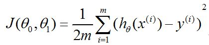
首先，我们根据线性回归模型：

得到成本函数：

其次，根据梯度下降法对回归变量theta中的每一个元素求偏导，并在赋予初始值后不断的更新theta值直至下降到最低点得到局部最小值，加入只有一个特征变量的情况下（不包括常数x0），则有按照如下方式更新theta的值：

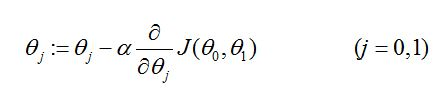
其中，类似于求偏导是把其他变量当作常数处理的一个过程，此时特征变量是已知值（常数）：

这里需要强调的是，x0作为常数theta0的的特征变量实际上全部是常数值1（无论是针对多少个样本（i=1....m））。

问题来了：

（1）怎么让你的最速下降模型朝着正确的方向下降，它一定会下降到局部最优点？

（2）学习速度alpha如何取值？

以上两个问题，依次做出解答：

针对问题（1），下图演示的是随着迭代次数的增加，成本函数的变化（我真是画图技术越来越好）：

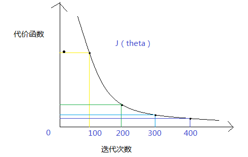
我们的目的是每一次迭代，成本函数的更新值只会越来越小，至于小到什么程度，打个比方：取最小误差值的边界值为eptheta=1/1000，一般读作10的负三次方。

针对问题（2），让alpha满足以下三个条件：

（i）取充分小的alpha使得J（theta）在每一次迭代之后变得更小；

（ii）如果取值太小，收敛到猴年马月；

（iii）如果取值太大，J（theta）很可能不能满足条件（i），甚至达到发散的结果，无终止的循环。。。

说的太多，画个简单明了的图给你们看看：

一般情况，我们会选择多个alpha的值：0.001，0.01，0.1，然后分别画出J（theta）与迭代次数之间的散点图，为梯度下降算法选择最合适的学习速度alpha。

罗嗦了半天，总算是把算法的整个过程描述出来了，还望各位觉得不对或者不熟悉的地方提出来，大家互相改进，那么接下来就是matlab中代价函数的实现（python突然罢工了，实际上numpy的编程跟matlab非常相似，相似到你无法想象的程度）：

代价函数：

function J = computeCost(X, y, theta) %COMPUTECOST Compute cost for linear regression %   J = COMPUTECOST(X, y, theta) computes the cost of using theta as the %   parameter for linear regression to fit the data points in X and y % Initialize some useful values m = length(y); % number of training examples % ====================== YOUR CODE HERE ====================== % Instructions: Compute the cost of a particular choice of theta %      You should set J to the cost. pred = X*theta;  % the prediction result sum = 0; for i = 1:m  % iterating from 1 to m  sum = sum+(pred(i) - y(i))^2; end J = 1/(2*m)*sum;  % compute the cost function % ========================================================================= end

梯度下降算法（只针对一个特征值）：

function [theta, J_history] = gradientDescent(X, y, theta, alpha, num_iters) %GRADIENTDESCENT Performs gradient descent to learn theta %   theta = GRADIENTDESENT(X, y, theta, alpha, num_iters) updates theta by  %   taking num_iters gradient steps with learning rate alpha % Initialize some useful values m = length(y); % number of training examples J_history = zeros(num_iters, 1);  % initializing all of J to zero before iteration for iter = 1:num_iters  % ====================== YOUR CODE HERE ======================  % Instructions: Perform a single gradient step on the parameter vector  %      theta.   %  % Hint: While debugging, it can be useful to print out the values  %    of the cost function (computeCost) and gradient here.  % =======This is my bug ======I just want to use jacobian but it seems  % =====something wrong, maybe because theta1 and theta2 are symbol variables=====  % syms theta1 theta2;  % temp_theta = [theta_1, theta_2];  % temp_rate = jacobian(J_history(iter), temp)'  % theta = theta - alpha * temp_rate * theta;  error = X * theta - y;  % the error between prediction and observation  delta = 1 / m * (error' * X)';  % the J's decrease slope  theta = theta - alpha * delta;  % ============================================================  % Save the cost J in every iteration   J_history(iter) = computeCost(X, y, theta); end end

前面提到“向量化”的概念，实际上上面的1到m个样本的迭代是直接借助矩阵中的向量运算的，改善代码如下：

sum=(pred - y)'*(pred - y);

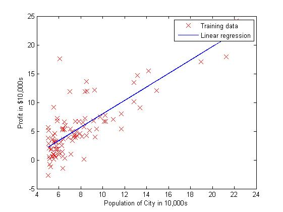
然后经过取学习速度alpha=0.01，1500次迭代后，拟合效果图的代码：

function plotData(x, y) %PLOTDATA Plots the data points x and y into a new figure  %   PLOTDATA(x,y) plots the data points and gives the figure axes labels of %   population and profit.  % ====================== YOUR CODE HERE ====================== % Instructions: Plot the training data into a figure using the  %               "figure" and "plot" commands. Set the axes labels using %               the "xlabel" and "ylabel" commands. Assume the  %               population and revenue data have been passed in %               as the x and y arguments of this function. % % Hint: You can use the 'rx' option with plot to have the markers %       appear as red crosses. Furthermore, you can make the %       markers larger by using plot(..., 'rx', 'MarkerSize', 10);  figure;                                 % open a new figure window plot(x, y, 'rx', 'MarkerSize', 10);     % plot the data ylabel('Profit in $10,000s')            % set the y-axis label xlabel('Population of City in 10,000s') % set the x-axis label  % ============================================================  end

拟合结果如下图所示：

机器学习《回归二》

总结：这里需要提到的另外一个算法是正则方程（“Normal Equation”）。我看到《机器学习实战》这本书直接给出的算法就是庸正则方程令误差为0，然后反过来求theta的值，这个时候有一个问题就是求逆，因为不是所有的矩阵都是有逆矩阵的，因此在python或者matlab中就给出了引入数值计算的函数直接求出“伪逆”来逼近真正的“逆”。因此，这个算法比较简单易行，针对较多的特征值的时候比较方便，比如说当样本数量m小于特征数量n的时候。

好啦，下周再见。

下期预告：局部加权线性回归～

正文到此结束