转载

MXNet实践

当下如此多的深度学习框架，为什么要选择MXNet？

MXNet是个深度学习的框架，支持从单机到多GPU、多集群的计算能力。对于其它深度学习框架来说，使用者得考虑什么时候开始计算，数据怎样同步。而这些在MXNet中都是“懒”操作（类似于Spark中的计算），MXNet等到资源合适就自己计算。

MXNet特点：

基于赋值表达式建立计算图，类似于Tensorflow、Teano、Torch和Caffe；
支持内存管理，并对两个不交叉的变量重复使用同一内存空间；
MXNet核心使用C++实现，并提供C风格的头文件。支持Python、R、Julia、Go和Javascript；
支持Torch；
支持移动设备端发布

命令式编程 vs 符号式编程

MXNet尝试将两种编程模式无缝的结合起来。命令式API作为一个接口暴露出来使用，类似于Numpy；符号表达式API提供用户像Theano和Tensorflow一样定义计算图。

命令式编程

NDarray编程接口，类似于Numpy.ndarray/Torch.tensor，主要是因为其提供张量运算（或称之为多维数组）；与Numpy不同的地方在于NDarray可以把对象的指针指向内存（CPU或GPU），它能自动的将需要执行的数据分配到多台gpu和cpu上进行计算，从而完成高速并行。

举个例子：在CPU和GPU上构建一个零张量。

import mxnet as mx cpu_tensor = mx.nd.zeros((10,), ctx=mx.cpu()) gpu_tensor = mx.nd.zeros((10,), ctx=mx.gpu(0))  类似于Numpy，MXNet可以做基本的数学计算。 ctx = mx.cpu() # which context to put memory on. a = mx.nd.ones((10, ), ctx=ctx) b = mx.nd.ones((10, ), ctx=ctx) c = (a + b) / 10. d = b + 1

MXNet实践

图1

与Numpy不同的地方在于，在数组上的操作都是惰性的，并且这些操作都会返回一个NDAarry实例（将来用于计算的）。MXNet真正厉害之处在于这些操作是如何计算的。一个计算计划生成后并不立即执行，而当此计算所依赖的数据都准备好才开始真正的计算。例如，计算D值时你需要知道B值而不需要C值，所以先计算B值。但计算C值和D值就无关顺序，并且可以利用并发计算。

在NDArray上读取值可以调用numpy_d = d.asnumpy()。这个调用是会触发d值的计算，然后转化成Numpy数组。

符号式编程

命令式编程有其优势，但其缺点在于计算都得提前知道计算完成的时间，并且得用户提前写好，而符号式编程试图解决这个问题。符号式程序的不同之处在于，当执行代码时，程序并没有产生真正的计算，而是生成了一张计算图/符号图（computation graph/symbolic graph）来描述整个计算过程。

举一个类似上面的例子：

import mxnet as mx a = mx.sym.Variable("A") # represent a placeholder. These can be inputs, weights, or anything else. b = mx.sym.Variable("B") c = (a + b) / 10 d = c + 1

当定义好符号图后，可以检查计算图输入和输出：

d.list_arguments() # ['A', 'B']  d.list_outputs() # ['_plusscalar0_output'] This is the default name from adding to scalar.

计算图允许图形操作：

# define input shapes inp_shapes = {'A':(10,), 'B':(10,)} arg_shapes, out_shapes, aux_shapes = d.infer_shape(**inp_shapes)  arg_shapes # the shapes of all the inputs to the graph. Order matches d.list_arguments() # [(10, ), (10, )]  out_shapes # the shapes of all outputs. Order matches d.list_outputs() # [(10, )]  aux_shapes # the shapes of auxiliary variables. These are variables that are not  trainable such as batch normalization population statistics. For now, they are save to ignore. # []

无状态图

不同于其它框架的，MXNet图是完全无状态的，计算图代表着有实参和输出的函数。在MXNet中，权重或者模型参数和数据输入（数据灌入）之间没有区别，它们都是计算图的实参。例如，一个逻辑回归计算图有三个实参：输入数据，权重变量，误差。

为了触发实际的图计算，可以调用Executor，然后绑定符号表达式和指定的输入变量。

input_arguments = {} input_arguments['A'] = mx.nd.ones((10, ), ctx=mx.cpu()) input_arguments['B'] = mx.nd.ones((10, ), ctx=mx.cpu()) executor = d.bind(ctx=mx.cpu(),                   args=input_arguments, # this can be a list or a  dictionary mapping names of inputs to NDArray                   grad_req='null') # don't request gradients  Executor申请所有需要的内存和临时变量来进行计算。一旦绑定好，Executor会一直 同一段内存空间做计算输入和输出。在执行一个符号表达式前，需要对所有的自由变 量进行赋值，执行完forward后softmax的输出。 import numpy as np # The executor executor.arg_dict # {'A': NDArray, 'B': NDArray}  executor['A'][:] = np.random.rand(10,) # Note the [:]. This sets the contents  of the array instead of setting the array to a new value instead of overwriting the variable. executor['B'][:] = np.random.rand(10,) executor.forward() executor.outputs # [NDArray] output_value = executor.outputs[0].asnumpy()

跟命令式编程类似，调用forward也是lazy的，在计算完成之前就回返回计算图。

计算流图比较重要的是它能根据相应的输入数据自动优化，这在backward函数中是自动进行的。Exector需要一定的空间来存放梯度输出，如下所示：

# allocate space for inputs input_arguments = {} input_arguments['A'] = mx.nd.ones((10, ), ctx=mx.cpu()) input_arguments['B'] = mx.nd.ones((10, ), ctx=mx.cpu()) # allocate space for gradients grad_arguments = {} grad_arguments['A'] = mx.nd.ones((10, ), ctx=mx.cpu()) grad_arguments['B'] = mx.nd.ones((10, ), ctx=mx.cpu())  executor = d.bind(ctx=mx.cpu(),                   args=input_arguments, # this can be a list or a dictionary  mapping names of inputs to NDArray                   args_grad=grad_arguments, # this can be a list or a dictionary  mapping names of inputs to NDArray                   grad_req='write') # instead of null, tell the executor to write  gradients. This replaces the contents of grad_arguments with the gradients computed.  executor['A'][:] = np.random.rand(10,) executor['B'][:] = np.random.rand(10,)  executor.forward() # in this particular example, the output symbol is not a scalar or loss symbol. # Thus taking its gradient is not possible. # What is commonly done instead is to feed in the gradient from a future computation. # this is essentially how backpropagation works. out_grad = mx.nd.ones((10,), ctx=mx.cpu()) executor.backward([out_grad]) # because the graph only has one output, only one output grad is needed.  executor.grad_arrays # [NDarray, NDArray]

命令式和符号式混合编程

MXNet真正厉害之处在于可以结合命令式编程和符号式编程两种风格。例如，你可以用符号表达式来构件一个神经网络，给定的batch_size，绑定一个executor来计算，然后用命令式API来计算梯度。所有这些操作都是等实际的数据到达才开始计算。

现在来点更复杂的例子：一个简单、全连接神经网络，带有一层隐藏层的MINIST。

MXNet实践

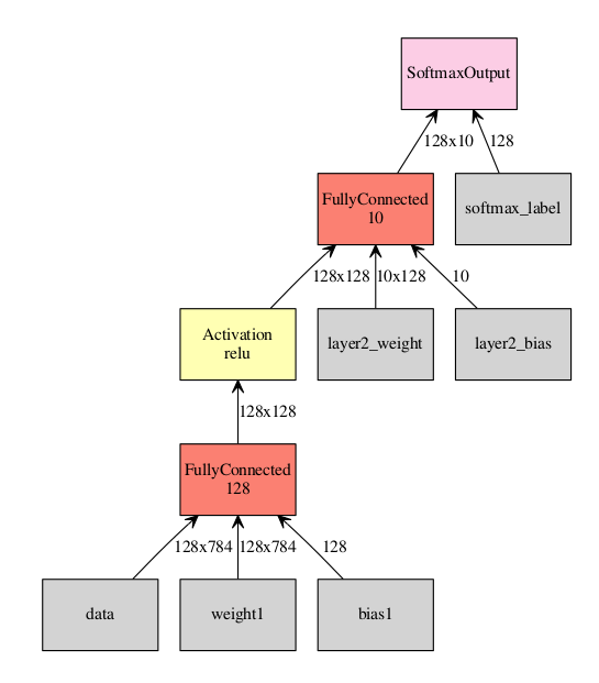
图2

import mxnet as mx import numpy as np # First, the symbol needs to be defined data = mx.sym.Variable("data") # input features, mxnet commonly calls this 'data' label = mx.sym.Variable("softmax_label")  # One can either manually specify all the inputs to ops (data, weight and bias) w1 = mx.sym.Variable("weight1") b1 = mx.sym.Variable("bias1") l1 = mx.sym.FullyConnected(data=data, num_hidden=128, name="layer1", weight=w1, bias=b1) a1 = mx.sym.Activation(data=l1, act_type="relu", name="act1")  # Or let MXNet automatically create the needed arguments to ops l2 = mx.sym.FullyConnected(data=a1, num_hidden=10, name="layer2")  # Create some loss symbol cost_classification = mx.sym.SoftmaxOutput(data=l2, label=label)  # Bind an executor of a given batch size to do forward pass and get gradients batch_size = 128 input_shapes = {"data": (batch_size, 28*28), "softmax_label": (batch_size, )} executor = cost_classification.simple_bind(ctx=mx.gpu(0),                                            grad_req='write',                                            **input_shapes) # The above executor computes gradients. When evaluating test data we don't need this. # We want this executor to share weights with the above one, so we will use bind # (instead of simple_bind) and use the other executor's arguments. executor_test = cost_classification.bind(ctx=mx.gpu(0),                                          grad_req='null',                                          args=executor.arg_arrays)  # initialize the weights for r in executor.arg_arrays:     r[:] = np.random.randn(*r.shape)*0.02  # Using skdata to get mnist data. This is for portability. Can sub in any data loading you like. from skdata.mnist.views import OfficialVectorClassification  data = OfficialVectorClassification() trIdx = data.sel_idxs[:] teIdx = data.val_idxs[:] for epoch in range(10):   print "Starting epoch", epoch   np.random.shuffle(trIdx)    for x in range(0, len(trIdx), batch_size):     # extract a batch from mnist     batchX = data.all_vectors[trIdx[x:x+batch_size]]     batchY = data.all_labels[trIdx[x:x+batch_size]]      # our executor was bound to 128 size. Throw out non matching batches.     if batchX.shape[0] != batch_size:         continue     # Store batch in executor 'data'     executor.arg_dict['data'][:] = batchX / 255.     # Store label's in 'softmax_label'     executor.arg_dict['softmax_label'][:] = batchY     executor.forward()     executor.backward()      # do weight updates in imperative     for pname, W, G in zip(cost_classification.list_arguments(), executor.arg_arrays, executor.grad_arrays):         # Don't update inputs         # MXNet makes no distinction between weights and data.         if pname in ['data', 'softmax_label']:             continue         # what ever fancy update to modify the parameters         W[:] = W - G * .001    # Evaluation at each epoch   num_correct = 0   num_total = 0   for x in range(0, len(teIdx), batch_size):     batchX = data.all_vectors[teIdx[x:x+batch_size]]     batchY = data.all_labels[teIdx[x:x+batch_size]]     if batchX.shape[0] != batch_size:         continue     # use the test executor as we don't care about gradients     executor_test.arg_dict['data'][:] = batchX / 255.     executor_test.forward()     num_correct += sum(batchY == np.argmax(executor_test.outputs[0].asnumpy(), axis=1))     num_total += len(batchY)   print "Accuracy thus far", num_correct / float(num_total)

MXNet提供大量的higher level APIs封装，减少直接使用forward模型的复杂性。例如，使用FeedForward类构建同样的模型，但是需要编写的代码量减小，编写代码也变的简单。

import mxnet as mx import numpy as np import logging logging.basicConfig(level=logging.INFO) logger = logging.getLogger(__name__) # get a logger to accuracies are printed  data = mx.sym.Variable("data") # input features, when using FeedForward this must be called data label = mx.sym.Variable("softmax_label") # use this name aswell when using FeedForward  # When using Forward its best to have mxnet create its own variables. # The names of them are used for initializations. l1 = mx.sym.FullyConnected(data=data, num_hidden=128, name="layer1") a1 = mx.sym.Activation(data=l1, act_type="relu", name="act1") l2 = mx.sym.FullyConnected(data=a1, num_hidden=10, name="layer2")  cost_classification = mx.sym.SoftmaxOutput(data=l2, label=label)  from skdata.mnist.views import OfficialVectorClassification  data = OfficialVectorClassification() trIdx = data.sel_idxs[:] teIdx = data.val_idxs[:]  model = mx.model.FeedForward(symbol=cost_classification,                              num_epoch=10,                              ctx=mx.gpu(0),                              learning_rate=0.001)  model.fit(X=data.all_vectors[trIdx],           y=data.all_labels[trIdx],           eval_data=(data.all_vectors[teIdx], data.all_labels[teIdx]),           eval_metric="acc",           logger=logger)