【特征工程】特征选择及mRMR算法解析
-
为什么?
(1)降低维度,选择重要的特征,避免维度灾难,降低计算成本
(2)去除不相关的冗余特征(噪声)来降低学习的难度,去除噪声的干扰,留下关键因素,提高预测精度
(3)获得更多有物理意义的,有价值的特征
-
不同模型有不同的特征适用类型?
(1)lr模型适用于拟合离散特征
(2)gbdt模型适用于拟合连续数值特征
(3)一般说来,特征具有较大的方差说明蕴含较多信息,也是比较有价值的特征
-
特征子集的搜索:
(1)子集搜索问题。
比如逐渐添加相关特征(前向forward搜索)或逐渐去掉无关特征(后向backward搜索),还有双向搜索。
缺点是,该策略为贪心算法,本轮最优并不一定是全局最优,若不能穷举搜索,则无法避免该问题。
该子集搜索策略属于最大相关(maximum-relevance)的选择策略。
(2)特征子集评价与度量。
信息增益,交叉熵,相关性,余弦相似度等评级准则。
-
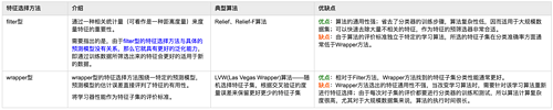
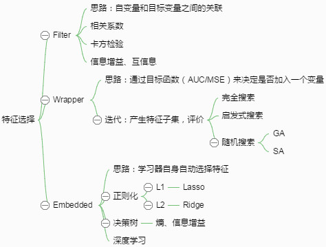
典型的特征选择方法
二、从决策树模型的特征重要性说起
决策树可以看成是前向搜索与信息熵相结合的算法,树节点的划分属性所组成的集合就是选择出来的特征子集。
(1)决策树划分属性的依据
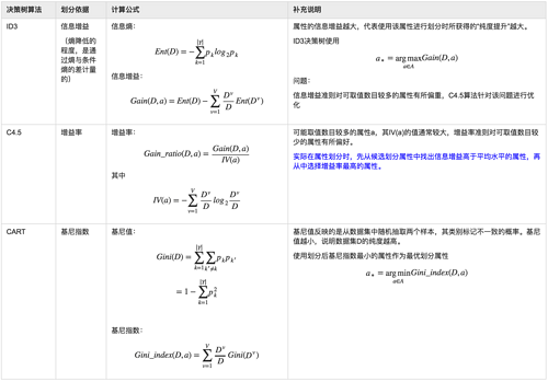
(2)通过gini不纯度计算特征重要性
不管是scikit-learn还是mllib,其中的随机森林和gbdt算法都是基于决策树算法,一般的,都是使用了cart树算法,通过gini指数来计算特征的重要性的。
比如scikit-learn的sklearn.feature_selection.SelectFromModel可以实现根据特征重要性分支进行特征的转换。
>>> from sklearn.ensemble import ExtraTreesClassifier
>>> from sklearn.datasets import load_iris
>>> from sklearn.feature_selection import SelectFromModel
>>> iris = load_iris()
>>> X, y = iris.data, iris.target
>>> X.shape
(150, 4)
>>> clf = ExtraTreesClassifier()
>>> clf = clf.fit(X, y)
>>> clf.feature_importances_
array([ 0.04...,  0.05...,  0.4...,  0.4...])
>>> model = SelectFromModel(clf, prefit=True)
>>> X_new = model.transform(X)
>>> X_new.shape
(150, 2)
(3)mllib中集成学习算法计算特征重要性的源码
在spark 2.0之后,mllib的决策树算法都引入了计算特征重要性的方法featureImportances,而随机森林算法(RandomForestRegressionModel和RandomForestClassificationModel类)和gbdt算法(GBTClassificationModel和GBTRegressionModel类)均利用决策树算法中计算特征不纯度和特征重要性的方法来得到所使用模型的特征重要性。
而这些集成方法的实现类都集成了TreeEnsembleModel[M <: DecisionTreeModel]这个特质(trait),即featureImportances是在该特质中实现的。
featureImportances方法的基本计算思路是:
- 针对每一棵决策树而言,特征j的重要性指标为所有通过特征j进行划分的树结点的增益的和
- 将一棵树的特征重要性归一化到1
- 将集成模型的特征重要性向量归一化到1
以下是源码分析:
deffeatureImportances[M <: DecisionTreeModel](trees: Array[M], numFeatures: Int): Vector = {
  val totalImportances = new OpenHashMap[Int, Double]()
  // 针对每一棵决策树模型进行遍历
  trees.foreach { tree =>
    // Aggregate feature importance vector for this tree
    val importances = new OpenHashMap[Int, Double]()
    // 从根节点开始,遍历整棵树的中间节点,将同一特征的特征重要性累加起来
    computeFeatureImportance(tree.rootNode, importances)
    // Normalize importance vector for this tree, and add it to total.
    //TODO:In the future, also support normalizing by tree.rootNode.impurityStats.count?
    // 将一棵树的特征重要性进行归一化
    val treeNorm = importances.map(_._2).sum
    if (treeNorm != 0) {
      importances.foreach { case (idx, impt) =>
        val normImpt = impt / treeNorm
        totalImportances.changeValue(idx, normImpt, _ + normImpt)
      }
    }
  }
  // Normalize importances
  // 归一化总体的特征重要性
  normalizeMapValues(totalImportances)
  // Construct vector
  // 构建最终输出的特征重要性向量
  val d = if (numFeatures != -1) {
    numFeatures
  } else {
    // Find max feature index used in trees
    val maxFeatureIndex = trees.map(_.maxSplitFeatureIndex()).max
    maxFeatureIndex + 1
  }
  if (d == 0) {
    assert(totalImportances.size == 0, s"Unknown error in computing feature" +
      s" importance: No splits found, but some non-zero importances.")
  }
  val (indices, values) = totalImportances.iterator.toSeq.sortBy(_._1).unzip
  Vectors.sparse(d, indices.toArray, values.toArray)
}
其中computeFeatureImportance方法为:
// 这是计算一棵决策树特征重要性的递归方法
defcomputeFeatureImportance(
    node: Node,
    importances: OpenHashMap[Int, Double]): Unit = {
  node match {
    // 如果是中间节点,即进行特征划分的节点
    case n: InternalNode =>
      // 得到特征标记
      val feature = n.split.featureIndex
      // 计算得到比例化的特征增益值,信息增益乘上该节点使用的训练数据数量
      val scaledGain = n.gain * n.impurityStats.count
      importances.changeValue(feature, scaledGain, _ + scaledGain)
      // 前序遍历二叉决策树
      computeFeatureImportance(n.leftChild, importances)
      computeFeatureImportance(n.rightChild, importances)
    case n: LeafNode =>
    // do nothing
  }
}
(4)mllib中决策树算法计算特征不纯度的源码
InternalNode类使用ImpurityCalculator类的私有实例impurityStats来记录不纯度的信息和状态,具体使用哪一种划分方式通过getCalculator方法来进行选择:
defgetCalculator(impurity: String, stats: Array[Double]): ImpurityCalculator = {
  impurity match {
    case "gini" => new GiniCalculator(stats)
    case "entropy" => new EntropyCalculator(stats)
    case "variance" => new VarianceCalculator(stats)
    case _ =>
      throw new IllegalArgumentException(
        s"ImpurityCalculator builder did not recognize impurity type:$impurity")
  }
}
以gini指数为例,其信息计算的代码如下:
@Since("1.1.0")
@DeveloperApi
override defcalculate(counts: Array[Double], totalCount: Double): Double = {
  if (totalCount == 0) {
    return 0
  }
  val numClasses = counts.length
  var impurity = 1.0
  var classIndex = 0
  while (classIndex < numClasses) {
    val freq = counts(classIndex) / totalCount
    impurity -= freq * freq
    classIndex += 1
  }
  impurity
}
以上源码解读即是从集成方法来计算特征重要性到决策树算法具体计算节点特征不纯度方法的过程。
三、最大相关最小冗余(mRMR)算法
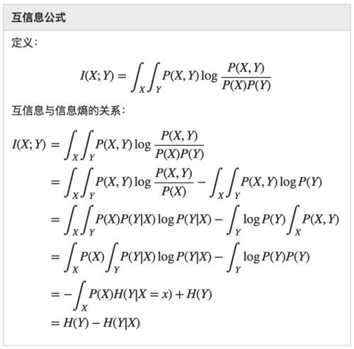
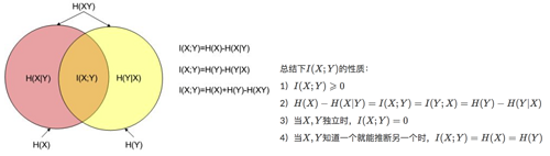
(1)互信息
互信息可以看成是一个随机变量中包含的关于另一个随机变量的信息量,或者说是一个随机变量由于已知另一个随机变量而减少的不确定性。互信息本来是信息论中的一个概念,用于表示信息之间的关系, 是 两个随机变量统计相关性的测度 。
(2)mRMR
之所以出现mRMR算法来进行特征选择,主要是为了解决通过最大化特征与目标变量的相关关系度量得到的最好的m个特征,并不一定会得到最好的预测精度的问题。
前面介绍的评价特征的方法基本都是基于是否与目标变量具有强相关性的特征,但是这些特征里还可能包含一些冗余特征(比如目标变量是立方体体积,特征为底面的长度、底面的宽度、底面的面积,其实底面的面积可以由长与宽得到,所以可被认为是一种冗余信息), mRMR算法就是用来在保证最大相关性的同时,又去除了冗余特征的方法 ,相当于得到了一组“最纯净”的特征子集(特征之间差异很大,而同目标变量的相关性也很大)。
作为一个特例,变量之间的相关性(correlation)可以用统计学的依赖关系(dependency)来替代,而互信息(mutual information)是一种评价该依赖关系的度量方法。
mRMR可认为是最大化特征子集的联合分布与目标变量之间依赖关系的一种近似。
mRMR本身还是属于filter型特征选择方法。
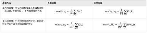
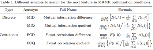
可以通过max(V-W)或max(V/W)来统筹考虑相关性和冗余性,作为特征评价的标准。
(3)mRMR的spark实现源码
mRMR算法包含几个步骤:
- 将数据进行处理转换的过程(注:为了计算两个特征的联合分布和边缘分布,需要将数据归一化到[0,255]之间,并且将每一维特征使用合理的数据结构进行存储)
- 计算特征之间、特征与响应变量之间的分布及互信息
- 对特征进行mrmr得分,并进行排序
/**
 * Perform a info-theory selection process.
 *
 * @param data Columnar data (last element is the class attribute).
 * @param nToSelect Number of features to select.
 * @param nFeatures Number of total features in the dataset.
 * @return A list with the most relevant features and its scores.
 *
 */
private[feature] defselectFeatures(
      data: RDD[(Long, Short)],
      nToSelect: Int,
      nFeatures: Int) = {

  // 特征的下标
  val label = nFeatures - 1
  // 因为data是(编号,每个特征),所以这是数据数量
  val nInstances = data.count() / nFeatures
  // 将同一类特征放在一起,根据同一key进行分组,然后取出最大值加1(?)
  val counterByKey = data.map({ case (k, v) => (k % nFeatures).toInt -> v})
        .distinct().groupByKey().mapValues(_.max + 1).collectAsMap().toMap

  // calculate relevance
  val MiAndCmi = IT.computeMI(
      data, 0 until label, label, nInstances, nFeatures, counterByKey)
  // 互信息池,用于mrmr判定,pool是(feat, Mrmr)
  var pool = MiAndCmi.map{case (x, mi) => (x, new MrmrCriterion(mi))}
    .collectAsMap()
  // Print most relevant features
  // Print most relevant features
  val strRels = MiAndCmi.collect().sortBy(-_._2)
    .take(nToSelect)
    .map({case (f, mi) => (f + 1) + "/t" + "%.4f" format mi})
    .mkString("/n")
  println("/n*** MaxRel features ***/nFeature/tScore/n" + strRels)
  // get maximum and select it
  // 得到了分数最高的那个特征及其mrmr
  val firstMax = pool.maxBy(_._2.score)
  var selected = Seq(F(firstMax._1, firstMax._2.score))
  // 将firstMax对应的key从pool这个map中去掉
  pool = pool - firstMax._1

  while (selected.size < nToSelect) {
    // update pool
    val newMiAndCmi = IT.computeMI(data, pool.keys.toSeq,
        selected.head.feat, nInstances, nFeatures, counterByKey)
        .map({ case (x, crit) => (x, crit) })
        .collectAsMap()

    pool.foreach({ case (k, crit) =>
      // 从pool里拿出第k个特征,然后从newMiAndCmi中得到对应的mi
      newMiAndCmi.get(k) match {
        case Some(_) => crit.update(_)
        case None =>
      }
    })

    // get maximum and save it
    val max = pool.maxBy(_._2.score)
    // select the best feature and remove from the whole set of features
    selected = F(max._1, max._2.score) +: selected
    pool = pool - max._1
  }
  selected.reverse
}
下面是基于互信息及mrmr的特征选择过程:
/**
 * Perform a info-theory selection process.
 *
 * @param data Columnar data (last element is the class attribute).
 * @param nToSelect Number of features to select.
 * @param nFeatures Number of total features in the dataset.
 * @return A list with the most relevant features and its scores.
 *
 */
private[feature] defselectFeatures(
    data: RDD[(Long, Short)],
    nToSelect: Int,
    nFeatures: Int) = {

  // 特征的下标
  val label = nFeatures - 1
  // 因为data是(编号,每个特征),所以这是数据数量
  val nInstances = data.count() / nFeatures
  // 将同一类特征放在一起,根据同一key进行分组,然后取出最大值加1(?)
  val counterByKey = data.map({ case (k, v) => (k % nFeatures).toInt -> v})
        .distinct().groupByKey().mapValues(_.max + 1).collectAsMap().toMap

  // calculate relevance
  val MiAndCmi = IT.computeMI(
      data, 0 until label, label, nInstances, nFeatures, counterByKey)
  // 互信息池,用于mrmr判定,pool是(feat, Mrmr)
  var pool = MiAndCmi.map{case (x, mi) => (x, new MrmrCriterion(mi))}
    .collectAsMap()
  // Print most relevant features
  // Print most relevant features
  val strRels = MiAndCmi.collect().sortBy(-_._2)
    .take(nToSelect)
    .map({case (f, mi) => (f + 1) + "/t" + "%.4f" format mi})
    .mkString("/n")
  println("/n*** MaxRel features ***/nFeature/tScore/n" + strRels)
  // get maximum and select it
  // 得到了分数最高的那个特征及其mrmr
  val firstMax = pool.maxBy(_._2.score)
  var selected = Seq(F(firstMax._1, firstMax._2.score))
  // 将firstMax对应的key从pool这个map中去掉
  pool = pool - firstMax._1

  while (selected.size < nToSelect) {
    // update pool
    val newMiAndCmi = IT.computeMI(data, pool.keys.toSeq,
        selected.head.feat, nInstances, nFeatures, counterByKey)
        .map({ case (x, crit) => (x, crit) })
        .collectAsMap()

    pool.foreach({ case (k, crit) =>
      // 从pool里拿出第k个特征,然后从newMiAndCmi中得到对应的mi
      newMiAndCmi.get(k) match {
        case Some(_) => crit.update(_)
        case None =>
      }
    })

    // get maximum and save it
    val max = pool.maxBy(_._2.score)
    // select the best feature and remove from the whole set of features
    selected = F(max._1, max._2.score) +: selected
    pool = pool - max._1
  }
  selected.reverse
}
具体计算互信息的代码如下:
/**
 * Method that calculates mutual information (MI) and conditional mutual information (CMI)
 * simultaneously for several variables. Indexes must be disjoint.
 *
 * @param rawData RDD of data (first element is the class attribute)
 * @param varX Indexes of primary variables (must be disjoint with Y and Z)
 * @param varY Indexes of secondary variable (must be disjoint with X and Z)
 * @param nInstances    Number of instances
 * @param nFeatures Number of features (including output ones)
 * @return  RDD of (primary var, (MI, CMI))
 *
 */
defcomputeMI(
    rawData: RDD[(Long, Short)],
    varX: Seq[Int],
    varY: Int,
    nInstances: Long,
    nFeatures: Int,
    counter: Map[Int, Int]) = {

  // Pre-requisites
  require(varX.size > 0)

  // Broadcast variables
  val sc = rawData.context
  val label = nFeatures - 1
  // A boolean vector that indicates the variables involved on this computation
  // 对应每个数据不同维度的特征的一个boolean数组
  val fselected = Array.ofDim[Boolean](nFeatures)
  fselected(varY) = true // output feature
  varX.map(fselected(_) = true) // 将fselected置为true
  val bFeatSelected = sc.broadcast(fselected)
  val getFeat = (k: Long) => (k % nFeatures).toInt
  // Filter data by these variables
  // 根据bFeatSelected来过滤rawData
  val data = rawData.filter({ case (k, _) => bFeatSelected.value(getFeat(k))})

  // Broadcast Y vector
  val yCol: Array[Short] = if(varY == label){
   // classCol corresponds with output attribute, which is re-used in the iteration
    classCol = data.filter({ case (k, _) => getFeat(k) == varY}).values.collect()
    classCol
  }  else {
    data.filter({ case (k, _) => getFeat(k) == varY}).values.collect()
  }

  // data是所有选择维度的特征,(varY, yCol)是y所在的列和y值数组
  // 生成特征与y的对应关系的直方图
  val histograms = computeHistograms(data, (varY, yCol), nFeatures, counter)
  // 这里只是对数据规约成占比的特征和目标变量的联合分布
  val jointTable = histograms.mapValues(_.map(_.toFloat / nInstances))
  // sum(h(*, ::))计算每一行数据之和
  val marginalTable = jointTable.mapValues(h => sum(h(*, ::)).toDenseVector)

  // If y corresponds with output feature, we save for CMI computation
  if(varY == label) {
    marginalProb = marginalTable.cache()
    jointProb = jointTable.cache()
  }

  val yProb = marginalTable.lookup(varY)(0)
  // Remove output feature from the computations
  val fdata = histograms.filter{case (k, _) => k != label}
  // fdata是特征与y的联合分布,yProb是一个值
  computeMutualInfo(fdata, yProb, nInstances)
}
计算数据分布直方图的方法:
private defcomputeHistograms(
    data: RDD[(Long, Short)],
    yCol: (Int, Array[Short]),
    nFeatures: Long,
    counter: Map[Int, Int]) = {

  val maxSize = 256
  val byCol = data.context.broadcast(yCol._2)
  val bCounter = data.context.broadcast(counter)
  // 得到y的最大值
  val ys = counter.getOrElse(yCol._1, maxSize).toInt

  // mapPartitions是对rdd每个分区进行操作,it为分区迭代器
  // map得到的是(feature, matrix)的Map
  data.mapPartitions({ it =>
    var result = Map.empty[Int, BDM[Long]]
    for((k, x) <- it) {
      val feat = (k % nFeatures).toInt; val inst = (k / nFeatures).toInt
      // 取得具体特征的最大值
      val xs = bCounter.value.getOrElse(feat, maxSize).toInt
      val m = result.getOrElse(feat, BDM.zeros[Long](xs, ys)) // 创建(xMax,yMax)的矩阵
      m(x, byCol.value(inst)) += 1
      result += feat -> m
    }
    result.toIterator
  }).reduceByKey(_ + _)
}
计算互信息的公式:
private defcomputeMutualInfo(
    data: RDD[(Int, BDM[Long])],
    yProb: BDV[Float],
    n: Long) = {

  val byProb = data.context.broadcast(yProb)
  data.mapValues({ m =>
    var mi = 0.0d
    // Aggregate by row (x)
    val xProb = sum(m(*, ::)).map(_.toFloat / n)
    for(i <- 0 until m.rows){
      for(j <- 0 until m.cols){
        val pxy = m(i, j).toFloat / n
        val py = byProb.value(j); val px = xProb(i)
        if(pxy != 0 && px != 0 && py != 0) // To avoid NaNs
          // I(x,y) = sum[p(x,y)log(p(x,y)/(p(x)p(y)))]
          mi += pxy * (math.log(pxy / (px * py)) / math.log(2))
      }
    }
    mi
  })
}
正文到此结束
热门推荐


相关文章

近期评论
-
主要用的是AI
-
博主的博客用的什么技术栈,内容都是干货,赞
-
-
https://www.liuhaihua.cn/archives/40657.html 这篇博客中的图片打不开了
-
不会英语啊。
-
-
-
-
-
Loading...
![[HBLOG]公众号](https://www.liuhaihua.cn/img/qrcode_gzh.jpg)