基于Tensorflow和TF-Slim图像分割示例

引言

在上一篇文章里(如何用TensorFlow和TF-Slim实现图像分类与分割)，我们介绍了如何截取图片的中央区域，然后用标准的分类模型对图片的类别进行预测。随后，我们又介绍了如何将网络模型改为全卷积模式，对整张图片进行预测。我们通过这种方法可以得到原始图片的一张降采样预测图 —— 降采样是由于网络结构含有最大池化层。这种预测图可以被视为一种全图的快速预测。你也可以把它看作是一种图像分割的方法，但并不算严格意义上的图像分割，因为标准网络模型是以图像分类的目标而训练得到的。为了实现真正的图像分割任务，我们需要在图像分割的数据集上重新训练模型，训练的方法参照Long等人发表的论文《Fully convolutional networks for semantic segmentation》。图像分割常用的两种数据集分别是：Microsoft COCO和PASCAL VOC。

在这篇文章里，我们将对预测图进行上采样，从而使得输出的图片与输入图片尺寸保持一致。值得注意的一点是不要把我们的方法与所谓的deconvolution混淆，它们分别是两种不同的操作方法。我们的方法准确的来说应该叫fractionally strided convolution，或者称之为微步长卷积吧。下文中，我们会适当介绍一些理论知识以便于理解。

也许大家现在会有一个问题：为什么我们需要用微步长卷积做上采样操作呢?为什么不能选用其它的上采样方法呢?简而言之：我们需要把上采样操作定义为模型的一层结构。为什么需要增加这一层呢?因为我们的训练数据上已经标注了图像分割的信息，我们需要根据这些信息来训练模型。众所周知，网络模型的每一层结构需要进行三种操作：前向传播、反向传播和参数更新。为了实现转置卷积的上采样，我们需要对这三种操作都给出定义，然后才能开始训练。

在文章的最后，我们将会实现上采样的过程，并且将结果与scikit-image库的实现做比较。具体说来，我们会实现《Fully convolutional networks for semantic segmentation》一文中的FCN-32图像分割网络。

本文是在jupyter notebook上完成的，所以大家也可以直接下载ipynb文件运行。

环境配置

为了成功运行文中的代码，请先输入一下命令，指定GPU和输入文件路径。可以参考上一篇文章的介绍。

from __future__ import division

import sys

import os

import numpy as np

from matplotlib import pyplot as plt

os.environ["CUDA_VISIBLE_DEVICES"] = '0'

sys.path.append("/home/dpakhom1/workspace/models/slim")

# A place where you have downloaded a network checkpoint -- look at the previous post

checkpoints_dir = '/home/dpakhom1/checkpoints'

sys.path.append("/home/dpakhom1/workspace/models/slim")

图片上采样

图片上采样是一种特殊的重采样方法。这篇论文中给出了重采样的定义：

重采样的思路就是用更多的样本(又称为插值或是上采样)或者更少的样本(又称为抽样或是降采样)来重建连续的信号。

换句话说，我们可以用已有的数据点估计连续信号，然后根据重建的信号采样得到新的样本点。就我们的问题而言，我们已有降采样的预测图 —— 它们就是信号重建的数据源。如果我们能估计出原始的信号，那么就可以从中采样出更多的样本，即实现了上采样。

我们强调“估计”是因为重建得到的原始连续信号效果可能并不太好。只有在某些条件限制下，信号才能被完全重建。根据香农采样定律，只有采样频率不小于模拟信号频谱中最高频率的2倍时，信号才能不失真地还原。

但是，信号还原的公式是什么?我们参考这篇文章中给出的公式：

s(x) = sum_n s(nT) * sinc((x-nT)/T)，

其中当x!=0时，sinc(x) = sin(pix)/(pix)，当x=0时 sinc(x)=1。

采样率为fs = 1/T，s(n*T)是连续信号s(x)的采样点，sinc(x)是重采样的核。

维基百科对上述公式做了完美的解释。

因此，我们需要将已有的数据点代入重采样核函数并求和(为了便于理解，忽略了一些细节)，以此来还原连续的信号。重采样的核函数并不一定用sinc函数。比如，也可以用双线性重采样核。这里给出了许多例子。上述解释的另外一个关键点是可以将核函数与Dirac脉冲信号序列做卷积运算，权重等于样本的值，它们在数学上是等价的。这两种等价的信号重建方式非常重要，因为它们有助于我们理解转置卷积的原理，以及每个转置卷积都有一种等价的卷积。

用scikit-image库内置的函数进行图像上采样运算。我们需要以此为参照，来验证我们双线性上采样的实现方式是正确的。这里是在合并到代码库之前的双线性上采样实现的验证过程。本文中的部分代码来源于此。接下去，我们会进行三倍上采样，也就是说输出图片的尺寸是输入图片的三倍。

%matplotlib inline

from numpy import ogrid, repeat, newaxis

from skimage import io

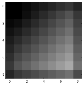
# Generate image that will be used for test upsampling

# Number of channels is 3 -- we also treat the number of

# samples like the number of classes, because later on

# that will be used to upsample predictions from the network

imsize = 3

x, y = ogrid[:imsize, :imsize]

img = repeat((x + y)[..., newaxis], 3, 2) / float(imsize + imsize)

io.imshow(img, interpolation='none')

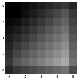
import skimage.transform

def upsample_skimage(factor, input_img):

# Pad with 0 values, similar to how Tensorflow does it.

# Order=1 is bilinear upsampling

return skimage.transform.rescale(input_img,

factor,

mode='constant',

cval=0,

order=1)

upsampled_img_skimage = upsample_skimage(factor=3, input_img=img)

io.imshow(upsampled_img_skimage, interpolation='none')

转置卷积

在Long的这篇论文里，他提到可以用微步长卷积(转置卷积)实现上采样。但是，首先要理解转置卷积的工作原理。我们先以普通的卷积为例，理解哪些参数会影响卷积结果的图片尺寸。如果我们想实现逆向操作该怎么办 —— 输入小尺寸的图片，输出大尺寸的图片，并且保留图片的连通性模式。下面是示例：

卷积是一类线性运算，因此它可以表示为矩阵的乘法。为了实现上述效果，我们只需对卷积运算的矩阵做转置。这种运算不再属于卷积，但仍能用卷积来表现。大家若想要更详细了解转置卷积的知识，推荐阅读这篇论文和这份指南。

所以，如果定义了双线性上采样核，并且对图片做了微步长卷积运算，我们就可以得到上采样的输出，它往往是网络结构的其中一层，能通过反向传播运算。对FCN-32网络，我们选用双线性上采样核为初始化，网络模型可以在反向传播过程中学会更合适的核。

为了便于理解代码，可以参考这个页面阅读。上采样的factor参数等于转置卷积的步长。上采样核的定义为：2 * factor - factor % 2。

我们在Tensorflow里用转置卷积运算来定义双线性插值。这部分运算放在CPU上，因为我们在后续篇幅中还会用到这段代码来进行内存开销较大的运算，因此不适合使用GPU。插值运算结束后，将我们的结果与sciki-image的运算结果做比较。

from __future__ import division

import numpy as np

import tensorflow as tf

def get_kernel_size(factor):

"""

Find the kernel size given the desired factor of upsampling.

"""

return 2 * factor - factor % 2

def upsample_filt(size):

"""

Make a 2D bilinear kernel suitable for upsampling of the given (h, w) size.

"""

factor = (size + 1) // 2

if size % 2 == 1:

center = factor - 1

else:

center = factor - 0.5

og = np.ogrid[:size, :size]

return (1 - abs(og[0] - center) / factor) * /

(1 - abs(og[1] - center) / factor)

def bilinear_upsample_weights(factor, number_of_classes):

"""

Create weights matrix for transposed convolution with bilinear filter

initialization.

"""

filter_size = get_kernel_size(factor)

weights = np.zeros((filter_size,

filter_size,

number_of_classes,

number_of_classes), dtype=np.float32)

upsample_kernel = upsample_filt(filter_size)

for i in xrange(number_of_classes):

weights[:, :, i, i] = upsample_kernel

return weights

def upsample_tf(factor, input_img):

number_of_classes = input_img.shape[2]

new_height = input_img.shape[0] * factor

new_width = input_img.shape[1] * factor

expanded_img = np.expand_dims(input_img, axis=0)

with tf.Graph().as_default():

with tf.Session() as sess:

with tf.device("/cpu:0"):

upsample_filt_pl = tf.placeholder(tf.float32)

logits_pl = tf.placeholder(tf.float32)

upsample_filter_np = bilinear_upsample_weights(factor,

number_of_classes)

res = tf.nn.conv2d_transpose(logits_pl, upsample_filt_pl,

output_shape=[1, new_height, new_width, number_of_classes],

strides=[1, factor, factor, 1])

final_result = sess.run(res,

feed_dict={upsample_filt_pl: upsample_filter_np,

logits_pl: expanded_img})

return final_result.squeeze()

upsampled_img_tf = upsample_tf(factor=3, input_img=img)

io.imshow(upsampled_img_tf)

# Test if the results of upsampling are the same

np.allclose(upsampled_img_skimage, upsampled_img_tf)

True

for factor in xrange(2, 10):

upsampled_img_skimage = upsample_skimage(factor=factor, input_img=img)

upsampled_img_tf = upsample_tf(factor=factor, input_img=img)

are_equal = np.allclose(upsampled_img_skimage, upsampled_img_tf)

print("Check for factor {}: {}".format(factor, are_equal))

Check for factor 2: True

Check for factor 3: True

Check for factor 4: True

Check for factor 5: True

Check for factor 6: True

Check for factor 7: True

Check for factor 8: True

Check for factor 9: True

上采样预测

将我们的上采样结果转为真正的预测内容。我们选用上一篇文章中用过的VGG-16模型进行分类，然后将上采样方法应用于低分辨率的模型预测结果上。

在运行下面的代码之前，我要先修改VGG-16模型代码的其中一行，防止它继续减小图片的尺寸。具体来说，要把7x7卷积层的padding选项改为SAME。对于作者来说，他们希望得到输入图片的唯一预测结果，而我们的图片分割任务并不需要到这一步，否则上采样得到的图片与输入图片的尺寸还是不一致。经过上述修改之后问题就解决了。

由于参数特别多，运行下面的代码会占用很多内存，大概15GB，所以要留有足够的空间。

%matplotlib inline

from matplotlib import pyplot as plt

import numpy as np

import os

import tensorflow as tf

import urllib2

from datasets import imagenet

from nets import vgg

from preprocessing import vgg_preprocessing

checkpoints_dir = '/home/dpakhom1/checkpoints'

slim = tf.contrib.slim

# Load the mean pixel values and the function

# that performs the subtraction

from preprocessing.vgg_preprocessing import (_mean_image_subtraction,

_R_MEAN, _G_MEAN, _B_MEAN)

slim = tf.contrib.slim

# Function to nicely print segmentation results with

# colorbar showing class names

def discrete_matshow(data, labels_names=[], title=""):

fig_size = [7, 6]

plt.rcParams["figure.figsize"] = fig_size

#get discrete colormap

cmap = plt.get_cmap('Paired', np.max(data)-np.min(data)+1)

# set limits .5 outside true range

mat = plt.matshow(data,

cmap=cmap,

vmin = np.min(data)-.5,

vmax = np.max(data)+.5)

#tell the colorbar to tick at integers

cax = plt.colorbar(mat,

ticks=np.arange(np.min(data),np.max(data)+1))

# The names to be printed aside the colorbar

if labels_names:

cax.ax.set_yticklabels(labels_names)

if title:

plt.suptitle(title, fontsize=15, fontweight='bold')

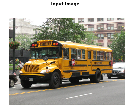
with tf.Graph().as_default():

url = ("https://upload.wikimedia.org/wikipedia/commons/d/d9/"

"First_Student_IC_school_bus_202076.jpg")

image_string = urllib2.urlopen(url).read()

image = tf.image.decode_jpeg(image_string, channels=3)

# Convert image to float32 before subtracting the

# mean pixel value

image_float = tf.to_float(image, name='ToFloat')

# Subtract the mean pixel value from each pixel

processed_image = _mean_image_subtraction(image_float,

[_R_MEAN, _G_MEAN, _B_MEAN])

input_image = tf.expand_dims(processed_image, 0)

with slim.arg_scope(vgg.vgg_arg_scope()):

# spatial_squeeze option enables to use network in a fully

# convolutional manner

logits, _ = vgg.vgg_16(input_image,

num_classes=1000,

is_training=False,

spatial_squeeze=False)

# For each pixel we get predictions for each class

# out of 1000. We need to pick the one with the highest

# probability. To be more precise, these are not probabilities,

# because we didn't apply softmax. But if we pick a class

# with the highest value it will be equivalent to picking

# the highest value after applying softmax

pred = tf.argmax(logits, dimension=3)

init_fn = slim.assign_from_checkpoint_fn(

os.path.join(checkpoints_dir, 'vgg_16.ckpt'),

slim.get_model_variables('vgg_16'))

with tf.Session() as sess:

init_fn(sess)

segmentation, np_image, np_logits = sess.run([pred, image, logits])

# Remove the first empty dimension

segmentation = np.squeeze(segmentation)

names = imagenet.create_readable_names_for_imagenet_labels()

# Let's get unique predicted classes (from 0 to 1000) and

# relable the original predictions so that classes are

# numerated starting from zero

unique_classes, relabeled_image = np.unique(segmentation,

return_inverse=True)

segmentation_size = segmentation.shape

relabeled_image = relabeled_image.reshape(segmentation_size)

labels_names = []

for index, current_class_number in enumerate(unique_classes):

labels_names.append(str(index) + ' ' + names[current_class_number+1])

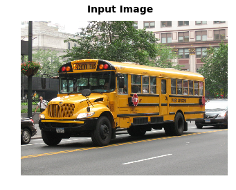
# Show the downloaded image

plt.figure()

plt.imshow(np_image.astype(np.uint8))

plt.suptitle("Input Image", fontsize=14, fontweight='bold')

plt.axis('off')

plt.show()

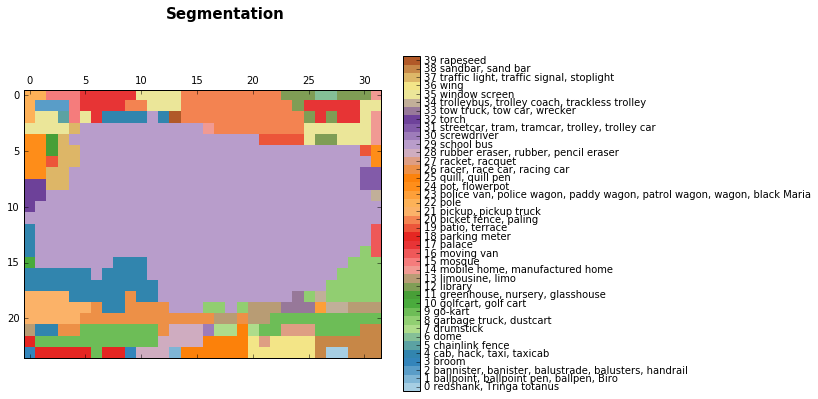
discrete_matshow(data=relabeled_image, labels_names=labels_names, title="Segmentation")

接着，我们用双线性上采样核对预测结果进行上采样操作。

upsampled_logits = upsample_tf(factor=32, input_img=np_logits.squeeze())

upsampled_predictions = upsampled_logits.squeeze().argmax(axis=2)

unique_classes, relabeled_image = np.unique(upsampled_predictions,

return_inverse=True)

relabeled_image = relabeled_image.reshape(upsampled_predictions.shape)

labels_names = []

for index, current_class_number in enumerate(unique_classes):

labels_names.append(str(index) + ' ' + names[current_class_number+1])

# Show the downloaded image

plt.figure()

plt.imshow(np_image.astype(np.uint8))

plt.suptitle("Input Image", fontsize=14, fontweight='bold')

plt.axis('off')

plt.show()

discrete_matshow(data=relabeled_image, labels_names=labels_names, title="Segmentation")

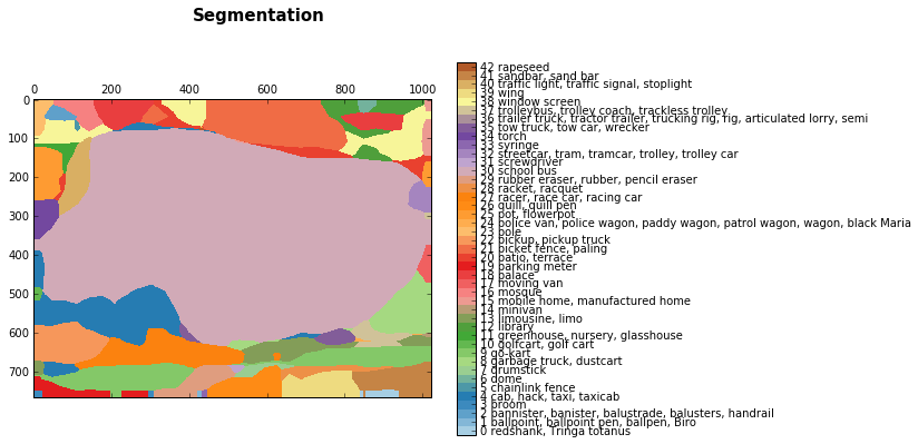
我们得到的结果混杂了很多噪音信息，但是我们基本上把校车给分割出来了。更确切的说，这并不是图像分割的结果，而是神经网络预测的分类标签所组成的区域。

总结

在本文中，我们介绍了转置卷积，特别是双线性差值的实现。我们对降采样的预测结果进行上采样还原，得到了整幅图片的预测类别。

另外，我们还发现对很多很多类别做图像分割时，会遇到内存消耗过大的问题，因此只能使用CPU计算。