利用Scikit-Learn和Spark预测Airbnb的listing价格
机器学习最有用的应用之一是预测客户的行为。这有广泛的范围:帮助顾客作出最优的选择(大多数是性价比最高的一个);让客户可以口碑相传你的产品;随着时间流逝建立忠诚的客户群体。当前顾客已不单单满足于从商品或者购物车中点击和购买,而是期待你提供智能化的推荐。
讲的很直白了。。。那实际情况下,你如何做到这些呢?让我们看下“分享经济”模式典范的Airbnb是如何做的,后续会从头到尾给出一个列子,使用Python和流行的 Scikit-Learn库 ,基于Airbnb已公开的 旧金山城市的数据 。
这次作者将用一种不同以往的方法来使用Apache Spark。常规情况下会使用 Spark MLlib 解决机器学习的问题。我们可以使用 spark-sklearn 集成开发包,扩展到多机器和多核运行,将会提高计算结果的速度和精度。
开始
我们基于listing属性开始listing价格预测。预测价格有几方面的应用:给客户提供建议的价格(价格太高或者太低都会显示提醒);帮助广告商做广告;提供数据分析给市场做决策。每个数据集包含以下几个感兴趣的项:
- listings.csv.gz:详细的listing数据,包含每个listing的各种属性,比如,卧室数目、浴室数目、位置等;
- calendar.csv.gz:每个listing的日历信息;
- reviews.csv.gz :listing的浏览数据;
- neighborhoods and GeoJSON files:同城邻居的地图和详细信息。
本列子提供了详细的使用Python编程的scikit-learn应用以及如何使用Spark进行交叉验证和调超参数。我们使用scikit-learn的线性回归方法,然后借助Spark来提高穷举搜素的结果和速度,这里面用到 GridSearchCV 和 GradientBoostingRegressor 方法。
扫描数据和清洗数据
首先,从MapR-FS文件系统加载listing.csv数据集,创建一个Pandas dataframe(备注:Pandas是Python下一个开源数据分析的库,它提供的数据结构DataFrame)。数据集大概包含7000条listing,每个listing 有90个不同的列,但不是每个列都有用,这里只挑选对最终的预测listing价格有用的几列。代码如下:
%matplotlib inline import pandas as pd import numpy as np from sklearn import ensemble from sklearn import linear_model from sklearn.grid_search import GridSearchCV from sklearn import preprocessing from sklearn.cross_validation import train_test_split import sklearn.metrics as metrics import matplotlib.pyplot as plt from collections import Counter LISTINGSFILE = '/mapr/tmclust1/user/mapr/pyspark-learn/airbnb/listings.csv' cols = ['price', 'accommodates', 'bedrooms', 'beds', 'neighbourhood_cleansed', 'room_type', 'cancellation_policy', 'instant_bookable', 'reviews_per_month', 'number_of_reviews', 'availability_30', 'review_scores_rating' ] # read the file into a dataframe df = pd.read_csv(LISTINGSFILE, usecols=cols)
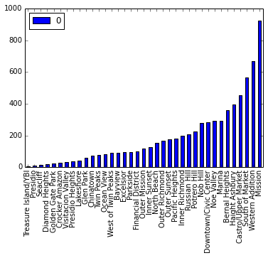
neighborhood_cleansed列是房主的邻居信息。你会看到这些信息分布不均衡,通过如下的图看出分布是个曲线,末尾的数量高,而靠左边非常少。总体来说,房主的邻居信息分布合理。
nb_counts = Counter(df.neighbourhood_cleansed) tdf = pd.DataFrame.from_dict(nb_counts, orient='index').sort_values(by=0) tdf.plot(kind='bar')
下面对数据进行按序清洗。
number_reviews'和 reviews_per_month两列看起来要去掉大量的NaN值(Python中NaN值就是NULL)。我们把reviews_per_month为NaN值的地方设置为0,因为在某些数据分析中这些数据是有意义的。
我们去掉那些明显异常的数据,比如,卧室数目、床或者价格为0的listing记录,并且删除那些NaN值的行。最后的结果集有5246条,原始数据集为7029条。
# first fixup 'reviews_per_month' where there are no reviews df['reviews_per_month'].fillna(0, inplace=True) # just drop rows with bad/weird values # (we could do more here) df = df[df.bedrooms != 0] df = df[df.beds != 0] df = df[df.price != 0] df = df.dropna(axis=0)
清洗的最后一步,我们把price列的值转换成float型数据,只保留卧室的数目等于1的数据。拥有一个卧室的数据大概有70%(在大城市,旧金山,这个数字还算正常),这里对这类数据进行分析。回归分析只对单个类型的数据进行分析,回归模型很少会和其他特征进行复杂的交互。为了对多个类型的数据进行预测,可以选择对不同的类型数据(比如,分为拥有2、3、4个卧室)单独进行建模,或者通过聚类对那些很容易区分开来的数据进行分析。
df = df[df.bedrooms == 1] # remove the $ from the price and convert to float df['price'] = df['price'].replace('[/$,)]','', / regex=True).replace('[(]','-', regex=True).astype(float) 类别变量处理
数据集中有几列包含分类变量。根据可能存在的值有几种处理方法。neighborhood_cleansed列是邻居的名字,string类型。scikit-learn中的回归分析只接受数值类型的列。对于这类变量,使用Pandas的get_dummies转换成虚拟变量,这个处理过程也叫“one hot”编码,每个listing行都包含一个“1”对应她/他的邻居。我们用类似的方法处理cancellation_policy和room_type列。
instant_bookable列是个boolean类型的值。 # get feature encoding for categorical variables n_dummies = pd.get_dummies(df.neighbourhood_cleansed) rt_dummies = pd.get_dummies(df.room_type) xcl_dummies = pd.get_dummies(df.cancellation_policy) # convert boolean column to a single boolean value indicating whether this listing has instant booking available ib_dummies = pd.get_dummies(df.instant_bookable, prefix="instant") ib_dummies = ib_dummies.drop('instant_f', axis=1) # replace the old columns with our new one-hot encoded ones alldata = pd.concat((df.drop(['neighbourhood_cleansed', / 'room_type', 'cancellation_policy', 'instant_bookable'], axis=1), / n_dummies.astype(int), rt_dummies.astype(int), / xcl_dummies.astype(int), ib_dummies.astype(int)), / axis=1) allcols = alldata.columns 接下来用Pandas的scatter_matrix函数快速的显示各个特征的矩阵,并检查特征间的共线性。本列子中共线性不明显,因为我们仅仅挑选列一小部分特征集,而且互相明显不相关。
scattercols = ['price','accommodates', 'number_of_reviews', 'reviews_per_month', 'beds', 'availability_30', 'review_scores_rating'] axs = pd.scatter_matrix(alldata[scattercols], figsize=(12, 12), c='red')
(点击放大图像)
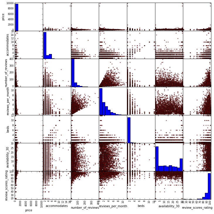
scatter_matrix的输出结果发现并没有什么明显的问题。最相近的特征应该是beds和accommodates。
开始预测
scikit-learn最大的优势是我们可以在相同的数据集上做不同的线性模型,这可以给我们一些调参的提示。我们开始使用其中的六种:vanilla linear regression, ridge and lasso regressions, ElasticNet, bayesian ridge和 Orthogonal Matching Pursuit。
为了评估这些模型哪个更好,我们需要一种对其进行打分,这里采用绝对中位误差。说到这里,很可能会出现异常值,因为我们没有对数据集进行过滤或者聚合。
rs = 1 ests = [ linear_model.LinearRegression(), linear_model.Ridge(), linear_model.Lasso(), linear_model.ElasticNet(), linear_model.BayesianRidge(), linear_model.OrthogonalMatchingPursuit() ] ests_labels = np.array(['Linear', 'Ridge', 'Lasso', 'ElasticNet', 'BayesRidge', 'OMP']) errvals = np.array([]) X_train, X_test, y_train, y_test = train_test_split(alldata.drop(['price'], axis=1), alldata.price, test_size=0.2, random_state=20) for e in ests: e.fit(X_train, y_train) this_err = metrics.median_absolute_error(y_test, e.predict(X_test)) #print "got error %0.2f" % this_err errvals = np.append(errvals, this_err) pos = np.arange(errvals.shape[0]) srt = np.argsort(errvals) plt.figure(figsize=(7,5)) plt.bar(pos, errvals[srt], align='center') plt.xticks(pos, ests_labels[srt]) plt.xlabel('Estimator') plt.ylabel('Median Absolute Error') 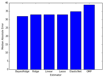
看下六种评估器得出的结果大体的相同,通过中位误差预测的结果是30到35美元。最终的结果惊人的相似,主要原因是我们未做任何调参。
接下来我们继续集成方法来获取更好的结果。集成方法的优势在于可以获得更好的结果,副作用便是超参数的“飘忽不定”,所以得调参。每个参数都会影响我们的模型,必须要求实验得出正确结构。最常用的方法是网格搜索法(grid search)暴力尝试所有的超参数,用交叉验证去找到最好的一个模型。Scikit-learn提供GridSearchCV函数正是为了这个目的。
使用GridSearchCV需要权衡穷举搜索和交叉验证所耗费的CPU和时间。这地方就是为什么我们使用Spark进行分布式搜索,让我们更快的去组合特征。
我们第一个尝试将限制参数的数目为了更快的得到结果,最后看下是不是超参数会比单个方法要好。
n_est = 300 tuned_parameters = { "n_estimators": [ n_est ], "max_depth" : [ 4 ], "learning_rate": [ 0.01 ], "min_samples_split" : [ 1 ], "loss" : [ 'ls', 'lad' ] } gbr = ensemble.GradientBoostingRegressor() clf = GridSearchCV(gbr, cv=3, param_grid=tuned_parameters, scoring='median_absolute_error') preds = clf.fit(X_train, y_train) best = clf.best_estimator_ 这次尝试的中位误差是23.64美元。已经可以看出用GradientBoostingRegressor比前面那次任何一种方法的结果都要好,没有做任何调优,中位误差已经比前面那组里最好的中位误差(使用BayesRidge()方法)还要少20%。
让我们看下每步boosting的误差,这样可以帮助我们找到迭代过程遇到的问题。
# plot error for each round of boosting test_score = np.zeros(n_est, dtype=np.float64) train_score = best.train_score_ for i, y_pred in enumerate(best.staged_predict(X_test)): test_score[i] = best.loss_(y_test, y_pred) plt.figure(figsize=(12, 6)) plt.subplot(1, 2, 1) plt.plot(np.arange(n_est), train_score, 'darkblue', label='Training Set Error') plt.plot(np.arange(n_est), test_score, 'red', label='Test Set Error') plt.legend(loc='upper right') plt.xlabel('Boosting Iterations') plt.ylabel('Least Absolute Deviation') 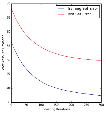
从曲线可以看出,曲线右边到200-250次迭代到位置仍然可以通过迭代获得好的结果,所以我们增加迭代次数到500。
接下来使用GridSearchCV进行各种超参数组合,这需要CPU和数小时。使用 spark-sklearn 集成 可以减少错误和时间。
from pyspark import SparkContext, SparkConf from spark_sklearn import GridSearchCV conf = SparkConf() sc = SparkContext(conf=conf) clf = GridSearchCV(sc, gbr, cv=3, param_grid=tuned_parameters, scoring='median_absolute_error')
至此,我们看下这种spark-sklearn 集成架构的优势。spark-sklearn 集成提供了跨Spark executor对每个模型进行分布式交叉验证;而Spark MLlib只是在集群间实际的机器学习算法间进行分布式计算。spark-sklearn 集成主要的优势是结合了scikit-learn 机器学习丰富的模型集合,这些算法虽然可以在单个机器上并行运算但是不能在集群间进行运行。
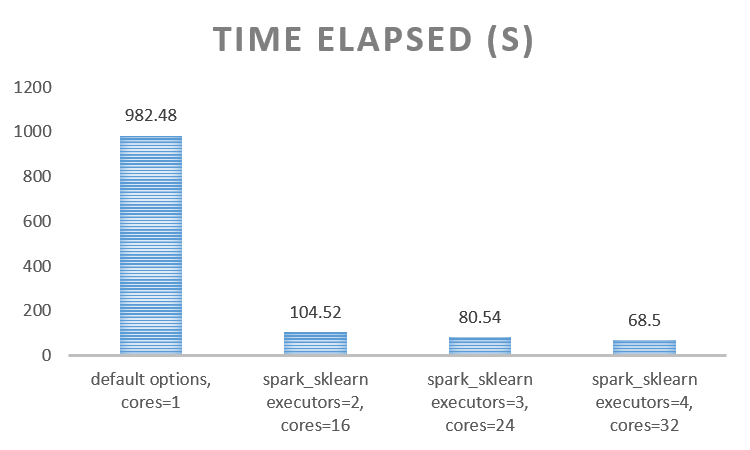
采用这种方法最后优化的中位差结果是21.43美元,并且还缩短了运行时间,如下图所示。集群为4个节点,以Spark YARN client模式提交,每个节点配置如下:
Machine: HP DL380 G6
Memory: 128G
CPU: (2x) Intel X5560
Disk: (6x) 1TB 7200RPM disks
最后让我们看下特征的重要性,下面显示特征的相对重要性。
feature_importance = clf.best_estimator_.feature_importances_ feature_importance = 100.0 * (feature_importance / feature_importance.max()) sorted_idx = np.argsort(feature_importance) pos = np.arange(sorted_idx.shape[0]) + .5 pvals = feature_importance[sorted_idx] pcols = X_train.columns[sorted_idx] plt.figure(figsize=(8,12)) plt.barh(pos, pvals, align='center') plt.yticks(pos, pcols) plt.xlabel('Relative Importance') plt.title('Variable Importance') (点击放大图像)
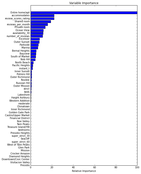
很明显的是有一些变量比其他变量更重要,最重要的特征是Entire home/apt。
结论
这个列子展示了如何使用spark-sklearn进行多变量来预测listing价格,然后进行分布式交叉验证和超参数搜索,并给出以下几点参考:
- GradientBoostingRegressor等集成方法比单个方法得出的结果要好;
- 使用GridSearchCV函数可以测试更多的超参数组合来得到更优的结果;
- 使用 spark-sklearn能更好节约CPU和时间,减少评估错误。
作者介绍
侠天,专注于大数据、机器学习和数学相关的内容,并有个人公众号:bigdata_ny分享相关技术文章。
正文到此结束
热门推荐


相关文章


Loading...
![[HBLOG]公众号](http://www.liuhaihua.cn/img/qrcode_gzh.jpg)